System Overview

The BenchBot is designed as a modular system to automate, monitor, and evaluate SLAM algorithms in simulated environments. This document provides a high-level overview of the system's architecture and design principles.

Modular Architecture

Concept: Frontend/Backend Separation

The system is not monolithic but divided into four independent pillars. This strict separation allows the execution engine to run in Headless mode (without a graphical interface) for Continuous Integration (CI/CD), while the GUI acts merely as a remote control.

The 4 Pillars

1. Frontend (GUI): Visualization and user control (PyQt5)
2. Backend (Runner): Orchestration and process management
3. Evaluation: Post-execution mathematical calculations
4. Infrastructure/Tools: Logging, report generation, simulator management

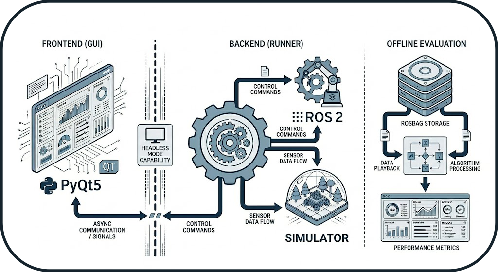
Frontend/Backend Separation

The Frontend/Backend separation ensures that the system can operate without a graphical interface, which is essential for CI/CD pipelines and server environments.

---

Design Patterns

The system uses several proven design patterns to ensure maintainability and extensibility:

1. State Machine (Orchestrator)

The orchestrator uses a Finite State Machine to manage the lifecycle of benchmarks deterministically.

Advantage: Ensures state transitions are controlled and data is only recorded when the system is stable.

2. Observer (Probes)

ROS 2 probes implement the Observer pattern to monitor the system status in real-time.

Advantage: Rapid problem detection and optimal startup (no fixed sleep()).

3. Adapter (Simulators)

Each simulator (Gazebo, O3DE) implements a common BaseSimulator interface.

Advantage: Adding a new simulator requires no modification to the orchestrator.

4. Strategy (Graceful Shutdown)

Process termination follows an escalation strategy (SIGINT → SIGTERM → SIGKILL).

Advantage: Clean process shutdown with fallback in case of hanging.

5. Deep Merge (Configuration)

Configuration resolution merges multiple layers according to a strict hierarchy.

Advantage: Full reproducibility with a single source of truth per run.

---

Data Flow

From Configuration File to Result

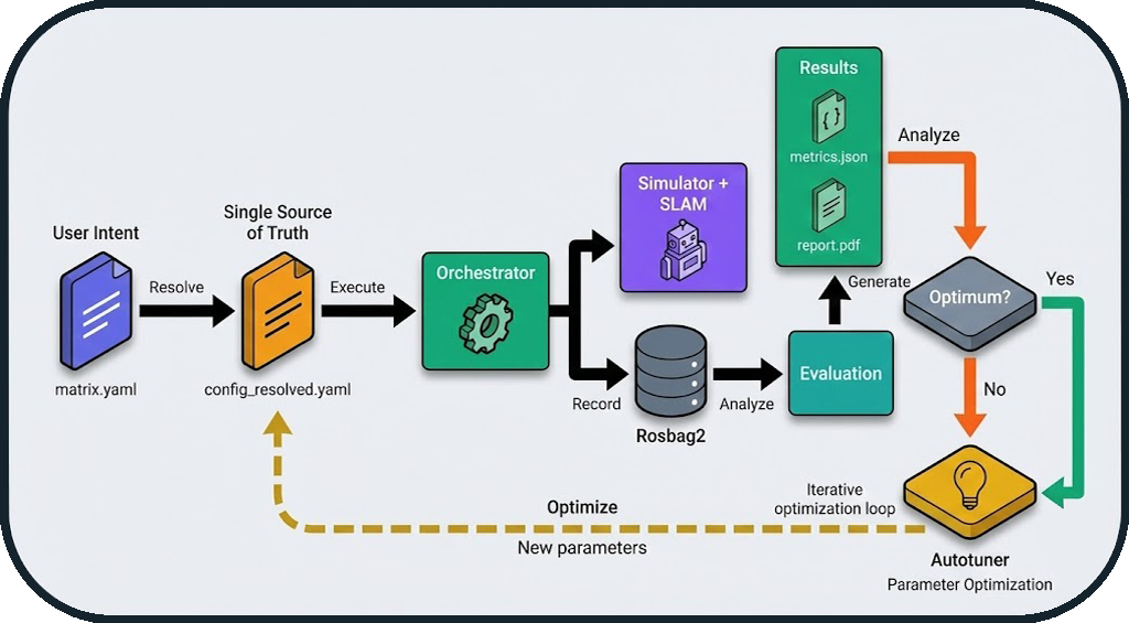
Key Steps

1. Configuration: Hierarchical merging of YAML files
2. Execution: Orchestration via state machine
3. Recording: ROS 2 data capture (rosbag2)
4. Evaluation: Metric calculation (IoU, SSIM, ATE, etc.)
5. Report: PDF generation with visualizations

Optimization Loop (Autotuner)

The diagram above also illustrates the automatic optimization loop:

Iterative Workflow:

1. After result generation, the system evaluates: "Optimum reached?"
2. If No: The autotuner analyzes metrics and proposes new parameters
3. Automatic Return: The new configuration is injected into config_resolved.yaml
4. New Run: The cycle restarts with optimized parameters
5. If Yes: The best configuration is saved (config_optimized.yaml)

Zero-Touch Optimization

This loop allows for automatic optimization of SLAM parameters (resolution, frequency, thresholds) without manual intervention between runs. The system can thus explore the parameter space and converge towards the optimal configuration for a given environment.

Example: Map resolution optimization

• Run 1: resolution=0.05m → IoU=0.82
• Run 2: resolution=0.025m → IoU=0.88 ✅
• Run 3: resolution=0.01m → IoU=0.87 (degradation)
• Result: Optimum = 0.025m (best quality/performance trade-off)

---

Typical User Workflow

From Need to Analysis: A Complete Benchmark Journey

This section describes the typical journey of a user wishing to evaluate a SLAM algorithm.

Phase 1: Preparation (5-10 minutes)

Objective: Define what to test

Actions: 1. Choose an environment (dataset): warehouse, office, maze 2. Select a SLAM algorithm: cartographer, slam_toolbox, rtabmap 3. Optional: Configure degradations (sensor noise, limited range)

Created File: matrix.yaml

matrix:
  include:
    - dataset: warehouse
      slam: cartographer
      degradation:
        enabled: true
        range_sensor:
          max_range: 8.0
          noise_std: 0.02

Key Decision: Which simulator to use? - Gazebo: Fast, stable, well-documented (recommended for starting) - O3DE: Realistic graphics, advanced physics (for visual tests)

Phase 2: Execution (2-5 minutes per run)

Objective: Launch the benchmark and collect data

Actions: 1. Launch via GUI: python -m gui.main → "Benchmark" Tab 2. Or via CLI: python -m runner.orchestrator --config matrix.yaml

Typical Timeline:

t=0s    : Environment cleanup + Config resolution
t=5s    : Simulator launch (Gazebo/O3DE)
t=15s   : SLAM launch + Navigation
t=20s   : Probe verification (topics, TF, services)
t=25s   : Warmup (initial SLAM convergence)
t=30s   : Start rosbag recording
t=90s   : End recording (duration: 60s)
t=95s   : Graceful shutdown (SIGINT → SIGTERM → SIGKILL)
t=100s  : Preliminary metrics generation

Output: Folder results/runs/RUN_YYYYMMDD_HHMMSS/ - config_resolved.yaml: Exact configuration used - rosbag2/: Recorded ROS 2 data - logs/: Detailed execution logs - metrics_partial.json: System metrics (CPU, RAM)

Phase 3: Evaluation (30 seconds - 2 minutes)

Objective: Calculate quality metrics

Actions: 1. Automatic after run (if enabled) 2. Or manual: python -m evaluation.metrics --run-dir results/runs/RUN_XXX

Calculated Metrics: - IoU (Intersection over Union): Global similarity with GT - SSIM (Structural Similarity): Structural coherence - ATE (Absolute Trajectory Error): Localization precision - Coverage: Percentage of environment explored - Wall Thickness: Quality of detected walls

Output: metrics.json with all metrics

Phase 4: Analysis (5-10 minutes)

Objective: Interpret results and compare

Actions: 1. Visualize in GUI: "Comparison" Tab 2. Generate PDF report: python -m tools.report_generator 3. Compare multiple runs: Automatic tables and charts

Deliverables: - report.pdf: Professional report with visualizations - Superimposed trajectory plots (GT vs SLAM) - Comparative maps (difference heatmaps) - Multi-run metric tables

Advanced Use Cases

Test Matrix

# Test 3 SLAM × 2 environments × 2 noise levels = 12 runs
matrix:
  include:
    - slam: [cartographer, slam_toolbox, rtabmap]
      dataset: [warehouse, office]
      degradation:
        enabled: [false, true]

Result: 12 automatic runs with global comparative report

Parameter Optimization

# Test different map resolutions
matrix:
  include:
    - slam: cartographer
      slam_params:
        resolution: [0.025, 0.05, 0.1]

Result: Identify optimal resolution (quality/performance trade-off)

---

System Guarantees

The BenchBot system offers several architectural guarantees:

Guarantee	Description	Mechanism
Reproducibility	Two identical runs produce the same results	Immutable configuration (config_resolved.yaml)
Robustness	No zombie processes	Isolation by groups (os.setsid)
Traceability	Complete logs for every run	Centralized logger + crash reports
Flexibility	Multi-simulator support	Adapter Pattern
Reliability	Optimal startup	Active probes (vs sleep())

---

Next Steps

To deepen your understanding:

• Orchestrator Architecture: State machine and probes details
• Evaluation Logic: Metrics (IoU, SSIM, ATE, Coverage)
• Tools: Simulators, GT map generation, PDF reports
• API Reference: Source code documentation